
Welcome back to our discussion of the math knowledge required to perform FAIR analyses with the RiskLens platform (spoiler alert: not much).
If you haven’t read Do I Need to Be a Math Nerd? Part 1 you’ll want to check that out first. In that article I discussed how much math you need to know to scope your analysis (zero, actually), and to collect data and make estimates (minimal, including the concept of a 90% confidence interval). In Part 2, we’ll discuss the rest of the analysis process: running the Monte Carlo simulation and interpreting the results.
David Musselwhite leads the training program at RiskLens
Running Your Analysis (Math Required: None, but Basic Understanding of Monte Carlo Simulation Is Recommended.)
Once you’ve entered your estimates for the relevant variables on the Loss Event Frequency and Loss Magnitude sides of the model, you’re ready to run those estimates through RiskLens that automatically invokes a Monte Carlo simulation to derive how much risk you have from the scenario. Technically it doesn’t take any math knowledge to click the “Run Analysis” button, but if you want to understand what’s being done behind the scenes we need to briefly discuss Monte Carlo simulation.
All Monte Carlo simulation does is evaluate the same formula thousands of times, varying the inputs to the formula based on data ranges that you define. This allows you to see a range of possible outcomes, and their relative probabilities, instead of just relying on a single point-estimate generated from evaluating the formula only once.
For a brief primer on Monte Carlo simulation, check out my video Monte Carlo 101 in 5 Minutes.
In a simplified/conceptual form, the formula the Monte Carlo simulation is evaluating starts with data on the two forms of loss…
- Primary loss, such as the direct cost of staff time to respond to a data breach and
- Secondary loss, such as cost of fines and judgments resulting from a data breach
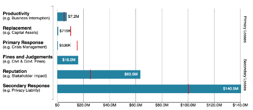
(Above) Forms of loss in a RiskLens analysis
…and adds them together to derive an estimated amount of risk, and looks like this:
(Loss Event Frequency * Primary Loss) + ((Loss Event Frequency * Secondary Loss Event Frequency) * Secondary Loss Magnitude) = Risk
See the FAIR Model for risk quantification explained on one page
To simplify further, the Monte Carlo simulation determines from your inputs how many primary loss events may occur, how much each of those will cost in primary losses, how many secondary loss events may occur, and how much each of those will cost in secondary losses. Adding those events and their associated losses together derives an estimated amount of risk.
By evaluating this formula thousands of times using different inputs drawn from the distributions you defined for the variables of the FAIR model, Monte Carlo simulation allows us to see the range of outcomes that are possible and their relative probabilities.
Presenting Results (Math Required: Basic Knowledge of Reading Graphs.)
The results of FAIR’s Monte Carlo simulations are most helpfully displayed as either a histogram or a loss exceedance curve.
Interpreting a histogram is relatively straightforward.
- The smallest amount of loss resulting from any Monte Carlo simulation is reported as the minimum and is represented in the bar that is farthest left on the horizontal axis.
- The largest amount of loss resulting from any Monte Carlo simulation is reported as the maximum and is represented in the bar that is farthest right on the horizontal axis.
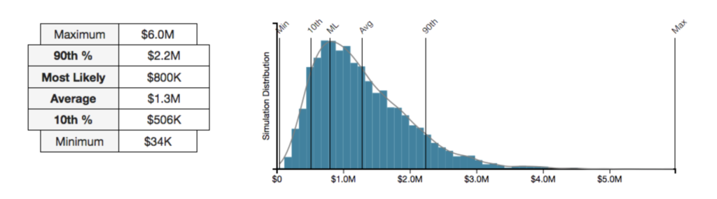
(Above) Histogram output from a RiskLens analysis
Assuming the accuracy of the estimates collected, we would not expect to see losses over the next year that are lower than the minimum value or higher than the maximum value.
Between the minimum and maximum there are other values of note: the 10th percentile, most likely, average, and 90th percentile, all of which can be helpful to report, and all of which are interpreted in this context the same way they would be in any other histogram.
- The 10th percentile is the value below which 10 percent of the simulated risk values fell, just as the 90th percentile is the value below which 90 percent of the simulated risk values fell.
- The most likely value represents the most likely amount of loss that can be expected based on the simulations.
- The average represents the mean amount of loss seen across all simulations. Keep in mind that the mean can be pulled to the right or left of the most likely value by simulated values at the high or low end. When your histogram is skewed in either direction, reporting the average amount of loss is not advisable.
Loss exceedance curves are in many ways superior to histograms for purposes of FAIR analysis. Instead of being forced to rely on the summary statistics outlined above, you get to choose the amount of money for which you want to know the probability of experiencing that amount of loss or more.
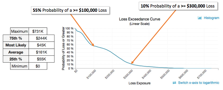
(Above) Loss Exceedance Curve output from RiskLens analysis
Here are the steps to interpreting a loss exceedance curve:
- Choose the amount of loss you’re interested in and locate it on the horizontal axis.
- Trace up from that amount on the horizontal axis until you reach the curve.
- Trace across to the left from the point at which you reach the curve until you reach the vertical axis.
- The value you land on the vertical axis tells you the probability of losing that amount of money or more based on the Monte Carlo simulation.
Related: What Does RiskLens Reporting Tell Me?
In summary…FAIR analysis with RiskLens does not take any advanced knowledge of math or statistics.
Some phases of the risk analysis process do not involve any math at all, and the ones that do can be understood with concepts that are typically a part of any Introductory Statistics course taught at the high school or college level.
For a more in-depth treatment of all of the concepts discussed in Parts 1 and 2 of this article, check out our online FAIR Analysis Fundamentals course.
FAIR is the international standard for quantitative cyber risk analysis. Membership in the FAIR Institute now exceeds 11,000 – and some 30% of the Fortune 100 use FAIR as an integral part of their risk management programs. Learn more about the growth of FAIR.