
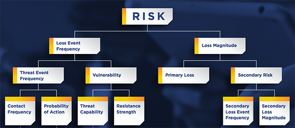
Read this blog post for a step-by-step guide on how to use critical thinking in quantitative cyber risk management when subject matter experts (SMEs) aren’t available to supply data. This is the first in a two-part series. Part 1 focuses on the left side of the FAIR™ model: Loss Event Frequency. Part 2 focuses on the right side of the model: Primary and Secondary Loss Magnitude (read it now).
There is no substitute for old fashioned human interaction, but with COVID-19 still at the forefront of everyone’s minds, finding ways to maintain productivity while remote is more important than ever. Over the last few weeks, RiskLens has published a number of tips on working from home as a risk analyst. In this post, we are focusing on how to make effective calibrated estimations even if your SMEs are unavailable.
4 Steps in Calibrated Estimation
 1. Start with the absurd
2. Eliminate highly unlikely values
**3. Reference what you know to narrow the range**
4. Use the equivalent bet method to gauge your confidence
Learn more: Calibrated Estimation for FAIR™ Cyber Risk Quantitative Analysis - Explained in 3 to 4 Minutes
Leverage Your Previous Cyber Risk Analysis Work
The third step of calibrated estimation (after "start with the absurd" and "eliminate highly unlikely values") is "reference what you know." One way to do this is referencing previous analyses. To do this, first consider how the analysis relates to other analyses you’ve done previously. Are there similar assets. threats, or effects? Is the data type the same? Does this method relate to one you’ve researched previously?
By thinking critically about other analyses, you can begin to find commonalities. From there you can evaluate the data point in question and consider how the two analyses relate.
As an example, imagine we are analyzing the risk associated with an outage of System A by an external malicious actor via ransomware. Before beginning our estimations, we begin by cataloging what we know:
- Internal system supporting critical business processes
- Two key departments in our organization rely on it to some extent daily
- To our knowledge, there are no known outage events of this type
Because there are no known loss events, we know it would more beneficial to estimate at Threat Event Frequency (attempts) and Vulnerability (susceptibility to attempts). Given that we are not the subject matter expert on this asset, we do not know how many times in a given year an external actor will attempt to cause an outage of this system. But based on previous analyses we know the most common method for this type of event is ransomware, which typically requires a foothold in the organization to deploy.
From our training we remember that in order for a threat event to occur, the actor has to be in a position to attempt to cause harm to our asset. Because of this, the proper way to model our Threat Event Frequency is the number of successful footholds in the organization that target System A.
Check Industry Data
In the spirit of referencing what we know, we think back to industry data we were reviewing recently. We were reading the 2019 Verizon Data Breach Investigations Report and know that ransomware is the second most prevalent type of malware behind C2 (command and control) and that 94% of malware is delivered via email.
Based on this information, we decide to focus on phishing and subsequent malware install as our delivery method. While we haven’t done an analysis on ransomware previously, we have analyzed confidentiality scenarios of internal systems, which used a foothold via malware as the method as well. Using this data, we know that the frequency of footholds in our environment is between once every five years (0.20) and once per year (1).

TIP:
When using a data point from another analysis as reference, it is important to ask yourself if the value would be the same, higher, or lower than the original.
You want to ensure you are applying an equal amount of rigor to this analysis as to the one you are referencing.
Estimate Threat Event Frequency
Keeping that tip in mind, we need to determine if we expect our threat event frequency in this scenario will be higher, lower, or the same as in the scenario referenced above. In this case, we consider that while ransomware is the second most common form of malware, the malware identified in the estimate above may not be ransomware at all or may be targeting a different asset.
With that thought in mind, we assume that our Threat Event Frequency is likely less than the estimate we are referencing. We estimate our Threat Event Frequency as between once every 10 years (0.10) and once every other year (0.50). We clearly document our thought process as well as the specific data points used from past analyses within our rationale to ensure our logic is transparent.
Estimate Vulnerability
Now that we have an estimate for the number of targeted attempts to cause an outage of System A by an external malicious actor via ransomware, we need to determine our susceptibility to those types of attempts (Vulnerability). Usually when we consider Vulnerability, we talk to our SME and make a list of all relevant controls and categorize each as green (effective, reduces Vulnerability) or red (ineffective, does not reduce Vulnerability).
In lieu of our SME, we go back to what we do know about our asset. It is an internal system with high criticality, meaning it is likely to be in one of the segmented areas of the network. From past analyses we know that this usually means there is an additional firewall that must be bypassed in order to get to the system. In the confidentiality scenarios referenced above, we were focusing on a system in the segmented area as well. In that example, Vulnerability was estimated as 75% - 90%, with the rationale that an actor sophisticated enough to access the network and circumvent the malware detection controls would likely be able to circumvent the remaining firewall as well.
We then begin considering if our Vulnerability would be the same, less than, or greater than the Vulnerability of the scenario referenced above.
We consider that in our analysis, it is possible that the workstation that was compromised in order to gain a network foothold happens to have access to System A. If that is the case, then this firewall would be virtually meaningless. Taking inventory of this information, we assume that our Vulnerability is likely equal to or greater than the Vulnerability of the scenario we referenced above. As such, we estimate that our Vulnerability is between 75% - 95%.
To Recap Our Estimates So Far:
Threat Event Frequency: 1/10 years (0.10) – 1/ 2 years (0.50)
Vulnerability: 75% - 90%
Check and Document Analysis Work
Our next step of the analysis is to think through the right side of the model but before we do, we want to double check all of our inputs and rationale. We go back to each estimate and ensure we have documented the thought process, information considered, relevant controls, assumptions, and any remaining areas of uncertainty. We know that before we can present this to leadership, we will need to conduct a QA session with relevant stakeholders from Infosec and the System A team and want to make sure we can clearly articulate our reasoning for that call.
To continue the example and learn how to reference what you know from previous analyses to estimate Primary and Secondary Loss Magnitude, read Part 2.