

Read this blog post for a step-by-step guide on how to use critical thinking in quantitative cyber risk management when subject matter experts (SMEs) aren’t available to supply data. This is the second in a two-part series…
The first part of this series (Gathering Frequency Data for FAIR Cyber Risk Analysis in Lockdown – Go with What You Know) focused on the left side of the FAIR™ model: Loss Event Frequency. As a recap, we considered the information we knew about our asset as well as previous analyses conducted and estimated ranges for both Threat Event Frequency and Vulnerability:
- Threat Event Frequency: 1/10 years (0.10) – 1/ 2 years (0.50)
- Vulnerability: 75% - 90%
This next part of our analysis focuses on the impact of a Loss Event, the right side of the model: Primary and Secondary Loss Magnitude.
See the FAIR model on one page
As with the example in Part 1, we will be focusing on the risk associated with an outage of System A by an external malicious actor via ransomware. Before we begin, we will again catalog what information we do have:
- Internal system supporting critical business processes
- Two key departments in our organization rely on it to some extent daily
- There are no known outage events of this type
We need to know the RTO (recovery time objective) of that system in order to determine the extent of the loss magnitude it would cause. We have never done an analysis on System A before, so we do not have that information. We have, however, done an analysis of an outage of System B and know the RTO of that system is 1-2 hours. We can then think critically about the two assets to determine if we expect the RTO of System A would be lower, higher, or the same as System B.
Based on what we know of System A, we believe it is considered a higher criticality than System B due to the processes it supports. As such, we assume that the RTO would be less than or equal to the RTO of System B. We estimate the RTO of System A is 0.5-2 hours.
 TIP:
TIP:
With more data points at your disposal you will gain more precision in your calibrated estimations. But even with little information, you can still inform an accurate range.
Learn more: Calibrated Estimation for FAIR™ Cyber Risk Quantitative Analysis – Explained in 3 to 4 Minutes
Using the same logic, we can use calibration to estimate ranges for other data points such as incident response hours, productivity losses, and secondary losses.
Estimate Incident Response Hours
To determine what we expect our incident response efforts to be, we take a look at the analyses we have done previously. We note that for scenarios related to availability, the incident response time tends to be approximately 2–4 times the RTO of the system for each person involved. We know that in the event involving an outage of System B by an insider, the incident response hours were 2–8 hours per person for a total of 8-10 people, or 16-80 hours total.
When thinking about whether our incident response hours would be the same, less than, or greater than the estimates referenced above, we consider how our scenario differs from those above. We realize that in the scenario referenced above, the outage was caused by a privileged insider whereas we are concerned about an external malicious actor. Assuming that the investigation efforts may be more thorough and time consuming for an external actor than for an internal actor, we expect our incident response hours will be higher than what was referenced in the prior example.
Based on this information, we estimate the incident response hours for System A are between 1 – 10 hours per person for a total of 8-12 people, or 8-120 hours total.
Estimate Productivity Loss
Next we consider the potential for productivity losses. We know that these are sometimes related to employees being unable to do their work and other times related to the inability to generate revenue from sales or services. In this case, we know that System A is internal facing and does not directly support the sales process so we do not believe there would be direct revenue loss.
We do know, however, that in the event involving an outage of System B, 100-500 employees had a 5% - 25% reduction in their productivity during the duration of the outage. Given that we know System A is more critical to core processes than System B, we assume that the impact to productivity would likely be higher. Additionally, based on the information we were given, we know that System A supports two main departments which have approximately 250-1,000 employees each.
Using this information, we assume that between 500-2,000 employees will have productivity impacts of 25% - 50% for a period of 0.5 – 2 hours. We use our known employee hourly wage of $75 - $200 to value their time.
Evaluate Secondary Losses
Knowing that System A is an internal only facing system, to evaluate secondary losses we consider other scenarios involving outages of internal systems. We determine that unless the system outage impacts downstream work which may eventually lead to an impact to customers, it is highly unlikely that secondary losses will occur. Thinking back to our FAIR Fundamentals training and focusing on probable vs. possible, we decide to estimate Secondary Loss Event Frequency and all secondary losses as $0.
Learn more: Understanding Secondary Loss
To recap our estimates:
Threat Event Frequency: 1/10 years (0.10) – 1/ 2 years (0.50)
Vulnerability: 75% - 90%
RTO: .5 – 2 hours
Incident Response Hours (Primary Response): 8 - 120 hours
Number of Employees Impacted: 500 - 2,000
Average Weighted Employee Hourly Wage: $75 - $200
Employee Productivity Impact (Primary Productivity): $65 - $2,000
Secondary Loss Event Frequency: Not Applicable - 0%
Secondary Loss Magnitude (All): Not Applicable - $0
Run the Analysis on the RiskLens Platform
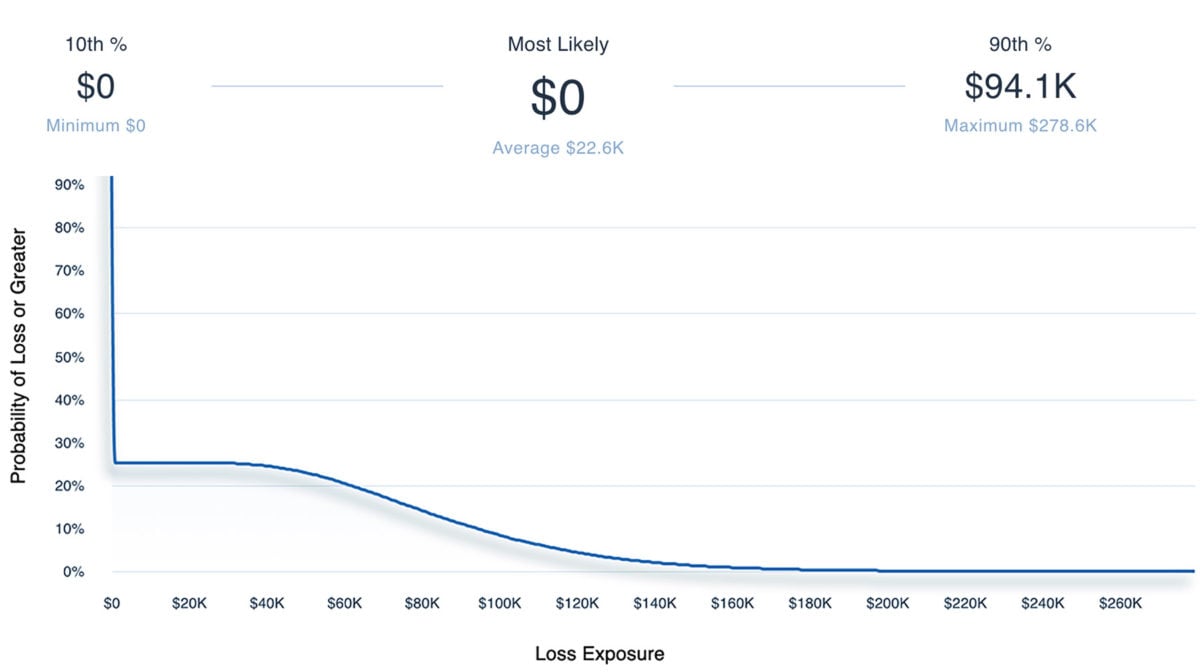
Having gathered all of the relevant estimates, we can enter the data into the RiskLens platform, using the guided functionality of the RiskLens platform. Then we use the platform to run 50,000 Monte Carlo simulations to estimate the probable range of annualized loss exposure in dollars as a loss exceedance curve. Below is an excerpt of the results we generated.
The 10th and 90th percentiles show where 80% of the simulated results fell. The Most Likely amount shows the annualized loss exposure that occurred most frequently in the simulated results. The $0 Most Likely figure represents that in the majority of simulated years, the Loss Event would not occur.
Interpret the Analysis Results to Determine Action Steps
In order to determine the appropriate remediation efforts required for this event, we compared the 90th percentile to our risk appetite. We know that the 90th percentile represents a “reasonable maximum” as there is only a 10% chance of exceeding this value in a given year. With a 90th percentile of under $100K, this scenario did not exceed our risk appetite of $1.5M. For now, this scenario does not require additional action, but we will follow-up in 6 months to re-evaluate.A couple more reminders before we go…
Rationale is always an important part of an analysis, but it is even more important when estimating in a silo. Be sure to clearly document your thought processes, any previous analyses and data points referenced, as well as any remaining uncertainty.
Learn more: Why Rationale Is Crucial in Cyber Risk Quantification
Just like documenting rationale, it is always best practice to conduct a Q/A of your analysis before finalizing. When working remote and estimating directly, this is more important than ever. If possible, schedule a web conference call to walk through your inputs and results with relevant stakeholders to confirm assumptions and make refinements as needed. At a minimum, you should provide the results and key inputs with rationale in email form to ensure all stakeholders have the opportunity to review.